Understanding Screen & World Space

Ryan McCombe
Every non-trivial game needs to represent positions in at least two different ways: where things are in the game world, and where they appear on the player's screen.
These different representation systems are called the world space and the screen space, and converting between them is a core skill in game development. In this lesson, we'll explore some of the main reasons why we need to work across multiple spaces, and how to transform our objects between them.
We’ll be using the Vec2 struct we created earlier in the course. A complete version of it is available below:
Vec2.h
#pragma once
#include <iostream>
struct Vec2 {
float x;
float y;
float GetLength() const {
return std::sqrt(x * x + y * y);
}
float GetDistance(const Vec2& Other) const {
return (*this - Other).GetLength();
}
Vec2 Normalize() const {
return *this / GetLength();
}
Vec2 operator*(float Multiplier) const {
return Vec2{x * Multiplier, y * Multiplier};
}
Vec2 operator/(float Divisor) const {
if (Divisor == 0.0f) { return Vec2{0, 0}; }
return Vec2{x / Divisor, y / Divisor};
}
Vec2& operator*=(float Multiplier) {
x *= Multiplier;
y *= Multiplier;
return *this;
}
Vec2& operator/=(float Divisor) {
if (Divisor == 0.0f) { return *this; }
x /= Divisor;
y /= Divisor;
return *this;
}
Vec2 operator+(const Vec2& Other) const {
return Vec2{x + Other.x, y + Other.y};
}
Vec2 operator-(const Vec2& Other) const {
return *this + (-Other);
}
Vec2& operator+=(const Vec2& Other) {
x += Other.x;
y += Other.y;
return *this;
}
Vec2& operator-=(const Vec2& Other) {
return *this += (-Other);
}
Vec2 operator-() const {
return Vec2{-x, -y};
}
};
inline Vec2 operator*(float M, const Vec2& V) {
return V * M;
}
inline std::ostream& operator<<(
std::ostream& Stream, const Vec2& V) {
Stream << "{ x = " << V.x
<< ", y = " << V.y << " }";
return Stream;
}Screen Space
Previously, we’ve been creating and managing our objects in screen space. Screen space is the coordinate system we use to position objects on the player’s screen.
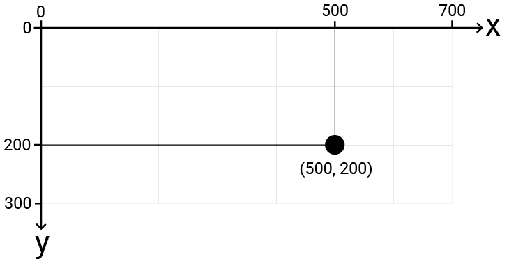
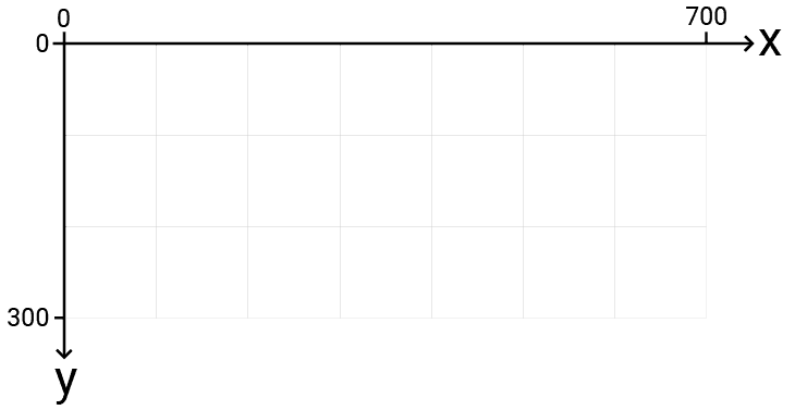
Our screen has been represented using the SDL_Surface corresponding to the SDL_Window where our game has been running. This surface configures the space it manages such that the top left corner is the origin, with increasing x values moving right and increasing y values moving down.
The space looks like with, with an example position highlighted:
When we start building more complex projects, this approach of programming everything in screen space has a few problems. For example:
- We don’t necessarily know the dimensions of the screen space at the time we’re writing our code. Users may be able to resize our window or, if our window is running in full screen, we may not know the resolution of that screen in advance.
- The screen-space coordinate system is rarely convenient. For example, we typically want downward movement to correspond with reducing values, but the SDL window’s coordinate system works in the opposite way. To move downwards within an
SDL_Surface, we need to increase theyvalue, which isn’t intuitive. - What is currently on the screen does not necessarily correspond to everything in our world. For example, many games involve the player controlling a character, and that character can only see a small part of the world at any given time. But the rest of the world is still there and the player may visit it in the future. As such, we need a space where objects in that world can continue to exist and be updated, even if they’re not being rendered to the screen right now.
Predictably, the space containing all the objects of our world, even when they’re not on the screen, is called the world space.
World Space
Most of our positioning and simulation are done within a coordinate system called the world space. When we create our game levels and worlds, the objects we position within them are in this world space.
We’re free to set this space up in whatever way is most convenient for the game we’re making. In 2D games, our world space typically uses an x dimension where increasing values correspond to moving right, and a y coordinate where increasing the value corresponds to moving up. In a 3D world space, the third dimension is typically labeled z and is perpendicular to both x and y.
In addition to choosing a coordinate system for our space, we also need to choose where the origin is - that is, what the x = 0, y = 0 position represents. A popular choice is to set up our space such that the origin represents the center of the world:
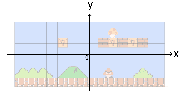
We can adjust our coordinate system and origin as needed based on the type of game and our preferences. For 2D games in particular, we typically don’t change the coordinate system from the previous example, but it may be more convenient to change what the origin position, represents.
We can adjust our coordinate system and origin as needed based on the type of game and our preferences. For 2D games in particular, we typically maintain the coordinate system (with increasing to the right and increasing upward) from the previous example, but it may be more convenient to change what the origin position represents.
For example, we could define the origin such that x = 0 aligns with the left edge of our level and for y = 0 to align with the bottom edge:
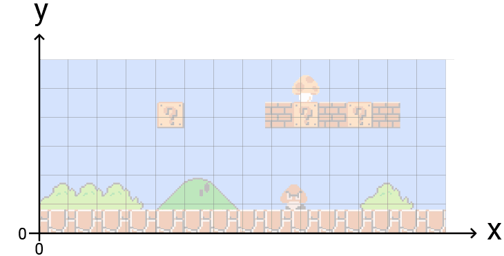
This is slightly less efficient as it means we won’t be using the "negative" range of our numeric types. However, that rarely matters for small levels, and not having to deal with negative numbers can make our lives slightly easier.
Transformations
Even though our objects are positioned in world space, the point of our game is ultimately to render those objects onto the player’s screen. So, we need some way to transform objects from their world space position to the corresponding screen space position.
This can be a challenge, as our spaces typically have different properties. There are three properties in particular where our spaces can differ:
- they can use different coordinate systems
- what the origin, , represents can have a different meaning
- they can have a different size
In most games, the world space and screen space differ across all three of these properties.
Example World Space and Screen Space
Later in this chapter, we’ll work with examples where our spaces are dynamically defined. For now, let’s work with a fixed example so we can establish the basics. We’ll imagine our world space looks like this:
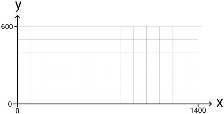
The key properties are:
- The
xdimension is horizontal, where increasing values correspond to moving right - The
ydimension is vertical, where increasing values correspond to moving up - The origin represents the bottom left of our world
- We want everything in our world space to be rendered to the screen, and everything in our space is within the range (0, 0) to (1400, 600)
Our screen space is the SDL_Surface associated with an SDL_Window. We’ll imagine the space looks like this:
The key properties are:
- The
xdimension has the same meaning as the world space - it is horizontal, where increasing values correspond to moving right - The
ydimension is also vertical, but increasing values correspond to moving down rather than up - The origin represents the top left of our screen
- The window’s dimensions are 700x300 - half the size of our world space
Transforming World Space to Screen Space
Later, we'll render our characters as images, so we'll represent the characters' positions at their top left corners. This corresponds to the x and y values we'd use in our SDL_Rect that controls where the image is blitted.
Despite our spaces being defined differently, we need our objects to be positioned in a visually consistent way across both spaces. That means we need to define logic that updates the x and y coordinates of an object in world space to what their equivalent values would be in screen space.
The following shows the start and end point of that process with two example objects - a dwarf and a dragon character:
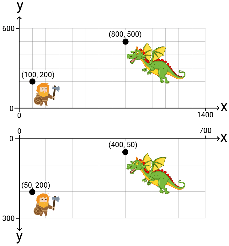
The challenge is determining what transformation logic to use, given how our screen space properties (coordinate system, size, and origin) differ from the world space properties.
Based on the properties we listed above for our example world and screen spaces, the transformation needs to:
- Account for the different size: Scale vectors down by 50% to account for the screen space being half the size of the world space. This corresponds to moving positions 50% closer to the origin.
- Account for the different coordinate system: Invert the
ycoordinates to account for the screen space’syaxis pointing in the opposite direction to the world space’s y axis. - Account for the the different origin: Increase
ycoordinates by 300 units (the height of the screen space) to account for the origin being at the top left of our screen space, rather than the bottom left. Given increasingyvalues corresponds to moving down in screen space, this step of our transformation will move (or "translate") our vectors down.
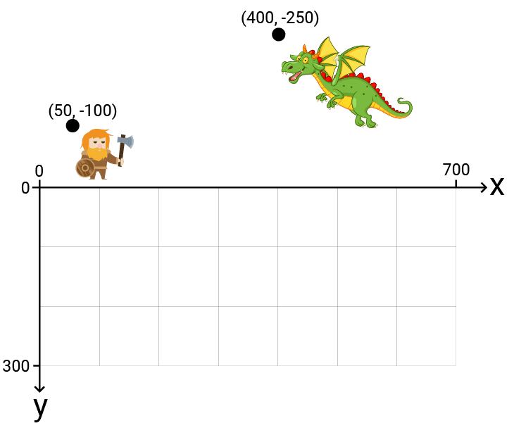
Let’s walk through this visually so we can better understand the logic we need to implement. First, let’s just place our characters in screen space, but using their world space coordinates without transformation. This helps us see the problem we need to solve:
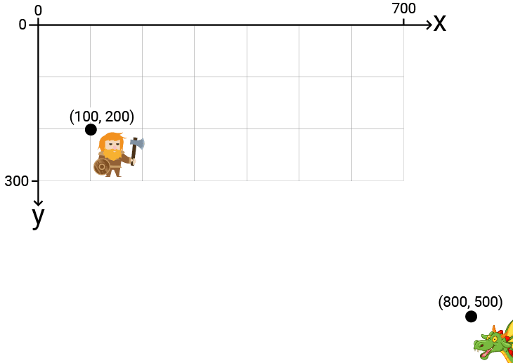
The horizontal position of our dwarf has shifted slightly, whilst our dragon is not even on the screen.
Step 1: Accounting for the Different Size
Let’s apply the first step of our transformation, multiplying all of the position vectors by . This scales them down to half of their current value, which is equivalent to moving them closer to the origin:
Step 2: Accounting for the Different Coordinate System
For step 2, we negate our objects’ vertical positions by multiplying their positions by . This moves them above the desired range and out of view, but we’ve made some progress - their positions relative to each other are now correct:
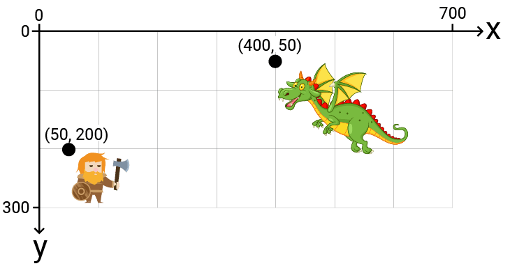
Step 3: Accounting for the Different Origin
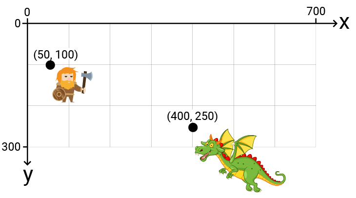
Finally, we perform step 3 of our transformation. We increase their components by which, in the screen space coordinate system, corresponds to moving the objects down by 300 units*.* This places our objects in their final, correct position:
Implementing our transformation in code could look like this:
Vec2 ToScreenSpace(const Vec2& Position) {
Vec2 ReturnValue{Position};
// 1: Scale every component by 50%
ReturnValue *= 0.5;
// 2: Invert the y component
ReturnValue.y *= -1;
// 3. Increase the y component. This
// corresponds to moving objects downwards
// in the screen space
ReturnValue.y += 300;
return ReturnValue;
}Or, equivalently:
Vec2 ToScreenSpace(const Vec2& Pos) {
return {
Pos.x * 0.5f,
(Pos.y * -0.5f) + 300
};
}Note that the ordering here is important. If we translated the vectors (step 3) before scaling and inverting the y axis (steps 1 and 2), then that translation would be done within the world space’s definition of y.
We can order it in that way if we want, but it means that our translation logic would need to be adjusted. For our example spaces, we could move objects down by equivalent amounts either by decreasing y values by 600 units in world space or by increasing y values by 300 units in screen space.
Whichever approach we use, we can transform some test points to ensure our logic is correctly mapping world space positions to equivalent screen space positions:
#include <iostream>
#include "Vec2.h"
Vec2 ToScreenSpace(Vec2&) {/*...*/}
int main() {
// A position in the center of
// the 1400x600 world space...
Vec2 P{700.0, 300.0};
// ...transformed to the center
// of the 700x300 screen space
std::cout << "[SCREEN SPACE]";
std::cout << "\nCenter: "
<< ToScreenSpace(P);
std::cout << "\nBottom Left: "
<< ToScreenSpace({0, 0});
std::cout << "\nTop Left: "
<< ToScreenSpace({0, 600});
std::cout << "\nBottom Right: "
<< ToScreenSpace({1400, 0});
std::cout << "\nTop Right: "
<< ToScreenSpace({1400, 600});
}[SCREEN SPACE]
Center: { x = 350, y = 150 }
Bottom Left: { x = 0, y = 300 }
Top Left: { x = 0, y = 0 }
Bottom Right: { x = 700, y = 300 }
Top Right: { x = 700, y = 0 }Advanced: Transformation Matrices
In higher budget games, these transformations tend to be implemented using transformation matrices and matrix multiplication - concepts from linear algebra. Linear algebra is the formal field of mathematics that studies vectors, spaces, and their transformations.
The linear algebra approach is more advanced, so we don’t cover it in detail in this course - we’ll continue to perform our transformations using regular C++ logic.
However, we’ll briefly introduce the alternative approach in this section, and we’ll also provide an additional, optional, lesson at the end of the chapter that goes a little deeper. That additional lesson will also implement these concepts using help from GLM, a popular library that provides math utilities for working with computer graphics.
The objectives and underlying theory of why we’re performing the transformations remain the same whichever approach we use - they key difference is the low-level mechanics of how the transformation is performed. Rather than creating a function to define the transformation, we can instead define a matrix - a two-dimensional grid of numbers that represents the transformation mathematically.
For example, we created a ToScreenSpace() function in the previous section, which defines a 2D transformation. It also provides the mechanism to perform that transformation - by calling the function with a position vector:
// Define the transformation
Vec2 ToScreenSpace(const Vec2& Pos) {
return {
Pos.x * 0.5f,
(Pos.y * -0.5f) + 300
};
}
// Perform the transformation
ToScreenSpace({700.0, 300.0});That same transformation can be defined using a matrix as follows:
We typically use a math library that help with this, ensuring the desired transformation is correctly represented by positioning appropriate values in appropriate positions within the matrix. We’ll cover this in more detail in our later lesson.
We can use this matrix to transform individual vectors, or we can arrange many vectors into a single matrix, where each vector is a column.
To make our vectors compatible with the transformation process, we need to add an additional component to them. So, for a 2D vector, we’d add a third component. This component has a value of if the vector represents a position and otherwise.
The five vectors we transformed in our previous example could be arranged in the following matrix:
Performing the transformation is then done by a matrix multiplication, a process that we again typically enlist the help of 3rd party library to implement, and we’ll cover in more detail later.
Matrix transformation involves multiplying our transformation matrix by the matrix of column vectors we want to transform:
The result of this multiplication is a matrix where each of our column vectors has been transformed:
Comparing this to our earlier program using the ToScreenSpace() function, we should see both approaches have the same effect:
Positions World Space -> Screen Space
Center: (700, 300) -> (350, 150)
Bottom Left: (0, 0) -> (0, 300)
Top Left: (0, 600) -> (0, 0)
Bottom Right: (1400, 0) -> (700, 300)
Top Right: (1400, 600) -> (700, 0)The matrix approach has a few advantages:
- We don’t need to write functions for our transformations, which saves time. Whilst our function was quite simple, transformations can get a lot more complex, especially when working with 3D spaces. Matrix techniques provide a general way to quickly create and represent transformations, including those that have rotations, scalings, shearings, and more.
- Much like vector math, the rules of matrix math have useful properties that can help us solve complex problems. For example, if we have multiple transformations represented as matrices, we can combine their effects to a single transformation by multiplying those matrices together.
- Computer hardware, especially the graphics processing unit (GPU), is highly optimized for performing matrix multiplication operations. This means that these approaches are typically more performant than providing our transformations as regular C++ functions.
Summary
In more complex games, objects are typically simulated in the world space, which has different properties to the screen space. To render our object, we need to derive their screen space position based on their world space position. The key takeaways from this lesson are:
- Screen space uses pixel coordinates with the origin at the top-left corner, while world space typically uses floating-point coordinates with various possible origins.
- When transforming between spaces, we must account for differences in scale, coordinate system orientation, and origin position.
- Transformations can be implemented as direct functions or using transformation matrices for more complex operations.


Ryan McCombe
Understanding Screen & World Space
Learn to implement coordinate space conversions in C++ to position game objects correctly on screen.

Game Dev with SDL2
Learn C++ and SDL development by creating hands on, practical projects inspired by classic retro games